Adding a cut in front of an NN
Contents
Adding a cut in front of an NN#
We’ve shown we can train a cut (or erf) and train a NN to separate signal from background. Can we do both? Here we will add two cuts in front of the same NN we used last time.
import jax
import jax.numpy as jnp
import numpy
import matplotlib.pyplot as plt
from samples import data_back, sig_avg, sig_width
from jax_helpers import erf, train
import haiku as hk
from typing import List, Optional

_ = plt.ion()
WARNING:absl:No GPU/TPU found, falling back to CPU. (Set TF_CPP_MIN_LOG_LEVEL=0 and rerun for more info.)
Load up the 2D data. This is identical to what we’ve done before.
key = jax.random.PRNGKey(1234)
signal_data = jax.random.multivariate_normal(key, jnp.asarray([1.5, 2.0]), jnp.asarray([[0.5, 0.2], [0.2, 0.5]]), [40000])
key, _ = jax.random.split(key)
background_data = jax.random.multivariate_normal(key, jnp.asarray([0.0, 0.0]), jnp.asarray([[9.0, 0.0], [0.0, 9.0]]), [40000])
Build the training and truth data. Keep the testing and training data the same, and the full data sample for now because we are lazy.
all_data = jnp.concatenate((signal_data, background_data))
all_truth = jnp.concatenate((jnp.ones(len(signal_data)), jnp.zeros(len(background_data))))

training_data = all_data
training_truth = all_truth

testing_signal = signal_data
testing_background = background_data
Building blocks for the network#
We will use the same network MLP as previous, but will add a parallel network that implements the cut. We’ll multiply the result of this network by the MLP result, so the cut can turn on-turn off the MLP output:
In order to do this, however, we have to build some new modules that are useful with haiku. We’ll need:
Multiplication -
n -> 1multiplies each row of the input vector together (implementes the \(*\) operators above).Selection Cut - implements the selection cut using the
erfwe used earlier in an earlier chapter.Concatenate - takes two other modules and just concatenates the outputs of each together. This is an infrastructure module and it is because we need the two selection cuts and the MLP to appear as a single row as input to the multiplication module.
Multiplication Module#
Implement a simple module that multiplies everything in a row together.
class MultiplyRow(hk.Module):
    'Multiply all elements of input together'

    def __init__(self, name='Multiply'):
        super().__init__(name=name)

    def __call__(self, x):
        'Multiply all elements of x'
        r = jnp.prod(x, axis=1)
        return r
Selection Cut#
We’ll use the code we used before in order to implement the error function, and allow us to properly set cuts. Given what we’ve learned, the initial value of the cuts are a bit tricky:
They need to be set somewhere in the bulk of the data
An easy stradegy might be to take the mean of the training data that is handed in initially as
xin the__call__method. See below for more discussion.
class Selection(hk.Module):
    """Apply a selection cut to each input, output is a weight,
    zero if the cut would reject, one if it would not"""

    def __init__(
        self, initial_cuts: Optional[List[float]] = None, name="SelectionCut"
    ):
        super().__init__(name=name)
        self._initial_cuts = initial_cuts

    def __call__(self, x):
        "Apply a selection cut for everything"

        # See if we have a decent set of initializers
        cuts_initial = (
            jnp.asarray(self._initial_cuts)
            if self._initial_cuts is not None
            else jnp.ones(x.shape[1])
        )
        assert (
            cuts_initial.shape[0] == x.shape[1]
        ), f"Incorrect number of initial cut values specified - need {x.shape[1]}"

        # Get the parameters to apply here
        cuts = hk.get_parameter(
            "cuts",
            shape=[x.shape[1]],
            dtype=jnp.float32,
            init=lambda shp, dtyp: cuts_initial,
        )

        # Next, apply the cut
        wts = (jax.lax.erf(x - cuts) + 1) / 2.0

        return wts
Concatenate#
This layer is odd because it takes as input two other layers, pushes the same inputs to each layer, and then returns the outputs concatinated together. So it doesn’t exactly follow the previous patterns (or standard haiku patterns for that matter). We will only implement this for starting from the same data - because I do not know how to do this otherwise.
If this had to be generalized, one could change the
__call__method to have two inputs, rather than listing them in thector- but that depends on weather the__call__is called under any other circumstances than network initalization.
class ModuleConcat(hk.Module):
    """Concatenate the outputs of two different networks that
    use the same data"""

    def __init__(self, layers: List[hk.Module], name="ModuleConcat"):
        super().__init__(name=name)
        self._layers = layers

    def __call__(self, x):
        layer_output = [layer(x) for layer in self._layers]

        c = jnp.concatenate(layer_output, axis=1)
        return c
Test the Selection Cut#
The error function has an issue that it has long plateaus when it is away from where it has “an effect”. If you do, the training grinds to a halt - which happened initally. So we can’t initialize with a value that is far outside where it might be cutting. In short - we have to choose our initial values carefully - we pick a randome spot along the x-axis and expect minimzation to get us to the right spot. Lets take a look at this, first by showing how the error function squared looks for a cut of -2.5 and the data is from -10 to 10.
select_model = hk.transform(lambda x: MultiplyRow()(Selection([-2.5, -2.5])(x)))
_ = select_model.init(key, training_data)
params = select_model.init(key, training_data)

cut_range_values = jnp.linspace(-10.0, 10.0, 101)
run_eval = [
    select_model.apply(params, key, jnp.ones([10, 2])*c)[0]
    for c in cut_range_values
]
plt.plot(cut_range_values, run_eval)
plt.xlabel('Value')
plt.xlabel('ERF^2 output (cut at -2.5)')
plt.show()
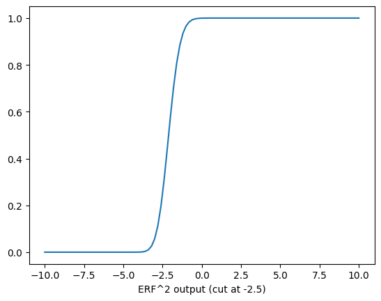
This is as expected from previous parts of the notebooks. Thinking about the derivative - if all your data sits out at 200, and the cut is down here at -2.5, the derivative will be zero. We can see that by looking at the derivative.
import optax

params = select_model.init(key, training_data)


def calc_value(params):
    preds = select_model.apply(params, key, training_data)
    preds = jax.nn.sigmoid(preds.squeeze())
    return optax.softmax_cross_entropy(preds, training_truth)


cut_range_values = jnp.linspace(-10.0, 10.0, 101)
cut_loss = [
    calc_value({"SelectionCut": {"cuts": jnp.asarray([v, v])}})
    for v in cut_range_values
]

plt.plot(cut_range_values, cut_loss)
plt.xlabel("Cut Value")
plt.ylabel("Loss")
plt.show()
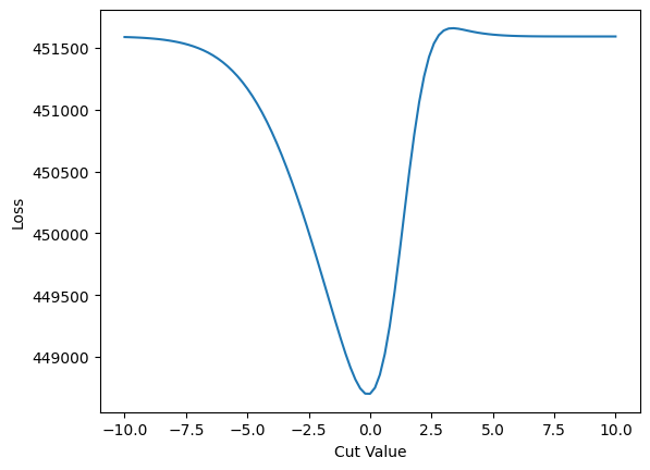
Note how it is basically flat around -10 and +10. If we were to extend the plot even further, it would look similar. In short - no gradient!
Note that we’ve taken a short cut here and used our knowledge of the training data to determine that -2.5 is good for both cuts. If this were really a new problem we’d need to evaluate this with each cut individually - like use the mean value. In reality any value where there is data should be fine - which suggests an easy way to start (say the median of each data for a straight up cut?).
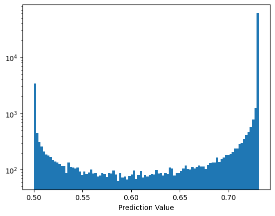
As further check the error function is doing what is expected, here are the two error functions multiplied together for two cuts on the training data (both signal and background):
preds = select_model.apply({'SelectionCut': {'cuts': jnp.asarray([-3.4, -3.6])}}, key, training_data)
preds = preds.squeeze()
preds = jax.nn.sigmoid(preds)
plt.hist(preds, bins=100)
plt.yscale('log')
plt.xlabel('Prediction Value')
plt.show()
Lets try a training the selection cuts and see how the training algorithm works with this.
select_params = train(
    model=select_model,
    key=key,
    epochs=1000,
    training_data=training_data,
    training_truth=training_truth,
)
NegLogLoss : 450008.03, epoch: 1
NegLogLoss : 449880.38, epoch: 100
NegLogLoss : 449746.75, epoch: 200
NegLogLoss : 449610.03, epoch: 300
NegLogLoss : 449472.38, epoch: 400
NegLogLoss : 449336.38, epoch: 500
NegLogLoss : 449205.22, epoch: 600
NegLogLoss : 449082.69, epoch: 700
NegLogLoss : 448972.72, epoch: 800
NegLogLoss : 448879.00, epoch: 900
NegLogLoss : 448803.69, epoch: 1000
print (select_params)
{'SelectionCut': {'cuts': DeviceArray([-0.6565423 , -0.51615274], dtype=float32)}}
The cuts are reasonable for the data, as can be seen on this scatter plot:
def plot_contour(data):
    counts,xbins,ybins,_ = plt.hist2d(data[:, 0], data[:, 1], bins=50, range=((-10, 10), (-10, 10)))
    plt.contour(counts.transpose(),extent=[xbins[0],xbins[-1],ybins[0],ybins[-1]], linewidths=3, cmap = plt.cm.rainbow, levels = [1,5,10,25,50,70,80,100])

plot_contour(signal_data)
plot_contour(background_data)
cut_values = select_params['SelectionCut']['cuts']
plt.axhline(cut_values[1])
plt.axvline(cut_values[0])
plt.show()
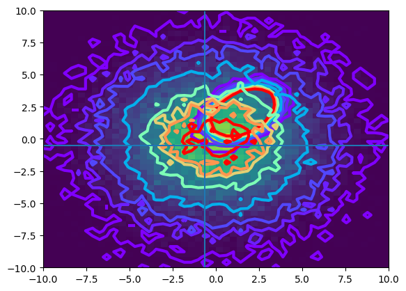
In order to get the training to work efficiently, I had add the Adam optimizer to the training loop above. That also meant what was taking a lot more than 20K training now takes about 1000 (and it hadn’t reached the optimal state by 20K either).
MLP + Selection Cut Network#
Build the forward network that combines all of this now.
def FeedForward(x):
    # The NN training
    mlp = hk.nets.MLP(output_sizes=[2,15,30,15,1])

    # The selection
    selection = Selection(initial_cuts=[0.0, 0.0])

    # Now the concat. Both these operate on the same input data (the tuple of
    # values) - which is required for this concat to work.
    combined = ModuleConcat([mlp, selection])

    # And then the multiply
    final = MultiplyRow()

    # And put them together in the proper way
    return final(combined(x))

model = hk.transform(FeedForward)
Train#
The training loop is the same as others we’ve used:
params = train(model=model,
    key = key,
    epochs = 40000,
    training_data=training_data,
    training_truth=training_truth,
    learning_rate = 0.0002)
NegLogLoss : 449200.66, epoch: 1
NegLogLoss : 442189.31, epoch: 4000
NegLogLoss : 440938.78, epoch: 8000
NegLogLoss : 440314.44, epoch: 12000
NegLogLoss : 439975.25, epoch: 16000
NegLogLoss : 439773.94, epoch: 20000
NegLogLoss : 439668.06, epoch: 24000
NegLogLoss : 439608.69, epoch: 28000
NegLogLoss : 439573.06, epoch: 32000
NegLogLoss : 439553.41, epoch: 36000
NegLogLoss : 439545.34, epoch: 40000
When compared to the straight-up training of the MLP found in the previous chapter, this is a lot slower:
Slower to get the loss down. The comparison can be made directly here - because the loss calculation is identical in the two cases.
Over all on a comparison laptop, it was 9.5 minutes to do 10K epochs here, and 2 minutes to do 2000 there - so about the same. At the end of 10K trainings however, the loss for this combined cut and MLP network is about at where the MLP only training was at 400 epochs. Even at the end of 40K iterations and 40 minutes, it doesn’t get as low a loss as the simple MLP training.
In short, using the multiplyer method may not be the most efficient way to train here. We can plot the output and look at where it pushes the cuts and the MLP on its own (I live `haiku), to see a bit more about what is going on.
First the raw output:
def plot_it(data, lbl):
    preds = model.apply(params, key, data)
    preds = preds.squeeze()
    # preds = jax.nn.sigmoid(preds)
    # preds = jnp.log(preds)
    plt.hist(preds, bins=100, label=lbl, alpha=0.5)


plot_it(signal_data, "signal")
plot_it(background_data, "background")
plt.yscale("log")
plt.xlabel("Prediction Values")
plt.legend()
plt.show()
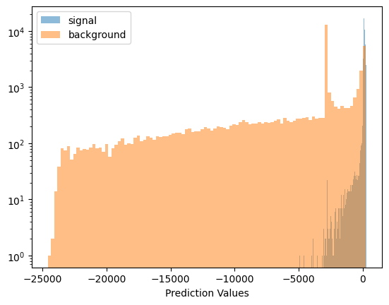
I had to shift from negative log loss function to optax’s softmax_cross_entropy in order to make this work. The reason is that when you hit values of about -45 or so for predicted values, your negative log heads off towards negative infinity.
Which brings up an interesting fact - compared to the plain old NN training, note that we go down to \(-25000\) in predictive values, where in the plain training it needs nothing beyond \(-40\) or so!
Examining the Training#
First, lets take a look at the cut parameters to see where they ended up (remember, they were initialized to 1).
trained_cut_values = params['SelectionCut']['cuts']
trained_cut_values
DeviceArray([-7.0540514, -7.112929 ], dtype=float32)
Look how far off the actual cut training this is!
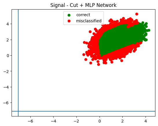
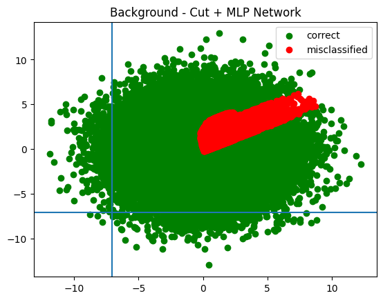
Lets look at this graphically, showing a scatter plot of good and bad. First the prediction!
def infer(data, p, m = model):
    test_preds = m.apply(p, key, data)
    test_preds = jax.nn.sigmoid(test_preds.squeeze())
    test_preds = (test_preds > 0.5).astype(jnp.float32)
    return test_preds

infer_signal = infer(testing_signal, params)
infer_background = infer(testing_background, params)
Next, plot the classified and mis-classified signal and background
def plot_inference(data, results, value, title, summary):
    good_data = data[results == value]
    plt.scatter(good_data[:, 0], good_data[:, 1], color='green', label='correct')
    bad_data = data[results != value]
    plt.scatter(bad_data[:, 0], bad_data[:, 1], color='red', label='misclassified')
    plt.title(f'{title} - {summary}')
    plt.legend()

def plot_in_and_out(i_signal, i_background, cuts = None, summary = ""):
    plot_inference(testing_signal, i_signal, 1.0, 'Signal', summary)
    if cuts is not None:
        plt.axhline(cuts[1])
        plt.axvline(cuts[0])
    plt.show()
    plot_inference(testing_background, i_background, 0.0, 'Background', summary)
    if cuts is not None:
        plt.axhline(cuts[1])
        plt.axvline(cuts[0])
    plt.show()

plot_in_and_out(infer_signal, infer_background, trained_cut_values, "Cut + MLP Network")
plot_contour(signal_data)
plot_contour(background_data)
cut_values = select_params['SelectionCut']['cuts']
plt.axhline(trained_cut_values[1])
plt.axvline(trained_cut_values[0])
plt.show()
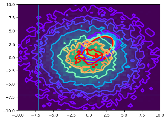
It looks way apart from any signal!
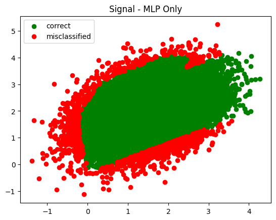
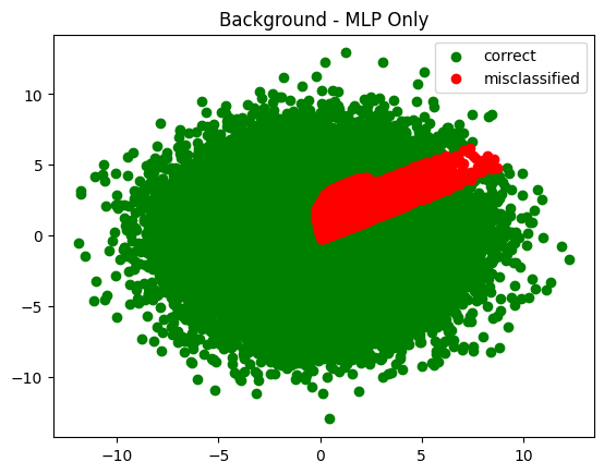
Lets take apart the performance of the two components (the cut and the NN), and look at their performance individually, but with the training values that are used here.
model_mlp_only = hk.transform(lambda x: hk.nets.MLP(output_sizes=[2,15,30,15,1])(x))
model_selection_only = hk.transform(lambda x: MultiplyRow()(Selection(initial_cuts=[0.0, 0.0])(x)))
def do_sig_b_infer(m):
    return (
        infer(testing_signal, params, m=m),
        infer(testing_background, params, m=m)
    )
infer_s_mlp, infer_b_mlp = do_sig_b_infer(model_mlp_only)
infer_s_sel, infer_b_sel = do_sig_b_infer(model_selection_only)
plot_in_and_out(infer_s_mlp, infer_b_mlp, summary='MLP Only')
plot_in_and_out(infer_s_sel, infer_b_sel, summary='Cuts Only')
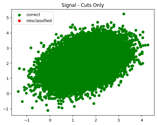
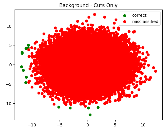
Fascinating in that it tried to push the cuts all the way out to the end - way past where there was any signal. I wonder what made it keep moving them?
The trend observed was generally this - each time I increased the number of training epochs the cuts were pushed further and further out.
