Gradient Descent

Now that we have a reasonable gradient vs the cut, lets use JAX to simply walk and find the zero of this function so we can find the “exact” maximum.

import jax
import jax.numpy as jnp
import numpy
import matplotlib.pyplot as plt
from jax_helpers import sig_sqrt_b

_ = plt.ion()

WARNING:absl:No GPU/TPU found, falling back to CPU. (Set TF_CPP_MIN_LOG_LEVEL=0 and rerun for more info.)

Our gradient is very very simple - no need to re-evaluate it every time around - there are no if statements, etc., in it that one might need to deal with each time. So we can evaluate it once.

grad = jax.grad(sig_sqrt_b)

cut_values = numpy.linspace(-10.0, 10.0, 100)
plt.plot(cut_values, numpy.array([grad(c) for c in cut_values]))
plt.xlabel('Cut Value')
plt.ylabel(r'Gradient vs cut value of the $S/\sqrt{B}$')
plt.axhline(0.0, color='black', linestyle='dashed')
plt.show()

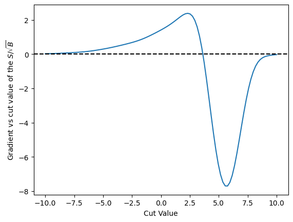
This does not look like a likelihood curve, sadly - so in order to help out any simplistic thing we code up here, we are going to just limit our cut_value a bit better, and then use that as the place to start our grad descent algorithm.

This is just relying on the idea we will have a likelihood that is well behaved and doesn’t have local minima.

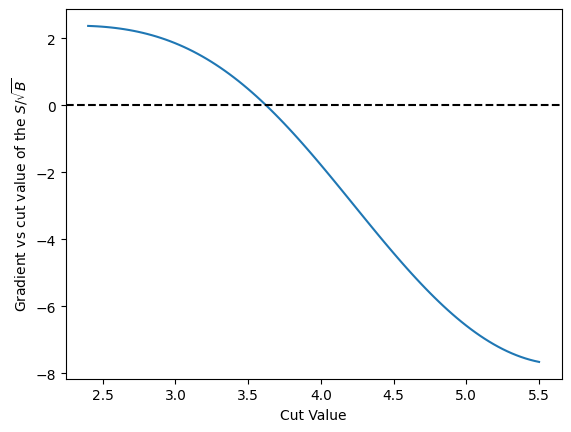
cut_values = numpy.linspace(2.4, 5.5, 100)
plt.plot(cut_values, numpy.array([grad(c) for c in cut_values]))
plt.xlabel('Cut Value')
plt.ylabel(r'Gradient vs cut value of the $S/\sqrt{B}$')
plt.axhline(0.0, color='black', linestyle='dashed')
plt.show()

Gradient Descent Loop

LEARNING_RATE = 0.06

def update_cut(c: float):
    'Run one iteration of the loop, and return a new cut value'

    g_value = grad(c)
    return c + g_value * LEARNING_RATE

c = 5.45
values = []
losses = []
loss = -1.0
for count in range(0, 50):
    loss = sig_sqrt_b(c)
    values.append(c)
    losses.append(loss)
    c = update_cut(c)
print(f'final cut is {c} with loss {loss}')

final cut is 3.624483346939087 with loss 20.89632797241211

fig, ax1 = plt.subplots() 

ax1.plot (range(0,50), losses, label=r'$S/\sqrt{B}$', color='blue')
ax1.set_ylabel(r'$S/\sqrt{B}$', color='blue')
ax1.tick_params(axis ='y', labelcolor = 'blue')
ax2 = ax1.twinx()
ax2.set_ylabel('Cut Value', color='orange')
ax2.plot (range(0, 50), values, label='Cut Value', color='orange')
ax2.tick_params(axis ='y', labelcolor = 'orange')
plt.xlabel('Training Iteration')
plt.show()

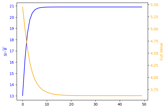
Ok - looks like it is basically done by 20 training iterations for that learning rate.