Using a ML-like Loss Function

In the end one likely wants to combine optimizing cuts with a more traditional ML-like set of cuts. Instead of the \(S/\sqrt{B}\) lets use the classification loss function that is more standard and see how that performs.

import jax
import jax.numpy as jnp
import numpy
import matplotlib.pyplot as plt
from samples import data_back, sig_avg, sig_width
from jax_helpers import erf

_ = plt.ion()

WARNING:absl:No GPU/TPU found, falling back to CPU. (Set TF_CPP_MIN_LOG_LEVEL=0 and rerun for more info.)

Create a complete array that has the values and the answers. The current signal and background samples aren’t the same size. This just makes the loss function harder to see. So - lets create a signal sample that is as big as the background sample.

data_sig = numpy.random.normal(sig_avg, sig_width, len(data_back))

training_data = jnp.concatenate((data_back, data_sig))
training_truth = jnp.concatenate((jnp.zeros(len(data_back)), jnp.ones(len(data_sig))))

Loss Function

A standard distance function:

def predict(c: float):
    'Predict if background or signal depending on the cut'
    return erf(training_data, c)

def loss(c: float):
    return jnp.sum((predict(c) - training_truth)**2)

cut_values = numpy.linspace(-10.0, 10.0, 100)
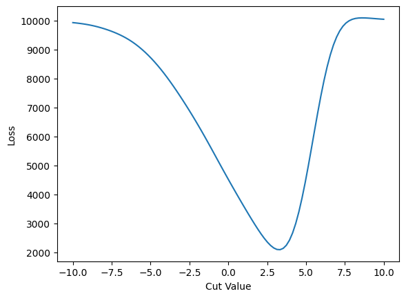
cut_loss = numpy.array([loss(c) for c in cut_values])

plt.plot(cut_values, cut_loss)
plt.xlabel('Cut Value')
plt.ylabel(r'Loss')
# plt.axvline(cut_values[max_index], color='green')
# plt.text(cut_values[max_index]+0.2, s_sqrt_b[max_index]/2.0, f'{cut_values[max_index]:0.3}', rotation=90)
plt.show()

Gradient

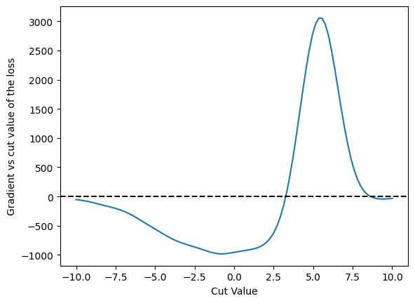
Look at the gradient of that function now

grad = jax.grad(loss)

plt.plot(cut_values, numpy.array([grad(c) for c in cut_values]))
plt.xlabel('Cut Value')
plt.ylabel(r'Gradient vs cut value of the loss')
plt.axhline(0.0, color='black', linestyle='dashed')
plt.show()

Gradient Descent Loop

Repeat the learning using gradient descent

LEARNING_RATE = 0.0005

def update_cut(c: float):
    'Run one iteration of the loop, and return a new cut value'

    g_value = grad(c)
    return c - g_value * LEARNING_RATE

c = 0.0
values = []
losses = []
l = -1.0
# log the cuts for tracking values during training
# will get used in next chapter.
with open('_cut.log', 'w') as out:
    for count in range(0, 50):
        l = loss(c)
        values.append(c)
        losses.append(l)
        c = update_cut(c)
        out.write(f'{c}\n')
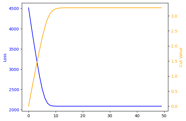
print(f'final cut is {c:0.3} with loss {l}')

final cut is 3.26 with loss 2082.857177734375

fig, ax1 = plt.subplots() 

ax1.plot (range(0,len(losses)), losses, label=r'$S/\sqrt{B}$', color='blue')
ax1.set_ylabel(r'Loss', color='blue')
ax1.tick_params(axis ='y', labelcolor = 'blue')
ax2 = ax1.twinx()
ax2.set_ylabel('Cut Value', color='orange')
ax2.plot (range(0, len(values)), values, label='Cut Value', color='orange')
ax2.tick_params(axis ='y', labelcolor = 'orange')
plt.xlabel('Training Iteration')
plt.show()

The 3.26 is close to the 3.62 that we found previously with \(S/\sqrt{B}\). However, the loss function is much better behaved and we did not have to choose our starting point for the cut carefully at all!

In a real experiment, we’d use the final likelihood in order to determine this value rather than a simple loss function. However, this will do for the rest of experiments.