This section will introduce some basic concepts:
- Making plots a Monte Carlo $Z \rightarrow ee$ electron $p_T$.
- Some simple filtering techniques (requiring the electron $p_T > 50$ GeV
- Some basics about what is going on under the hood
The following packages and methods are required for our work below.
# Because we aren't working from pypi yet...
import sys
sys.path = ['..'] + sys.path

from hep_tables import xaod_table, make_local
from func_adl import EventDataset
import matplotlib.pyplot as plt

# Make figures a size we can see
plt.rcParams.update({'figure.figsize':(7,5), 'figure.dpi':100})
Everything has to start from a dataset. For this work here (and further on) we'll use a $Z \rightarrow ee$ MC dataset from ATLAS. This is in the binary xAOD format, and is on rucio, and is contains 17 files.
dataset = EventDataset('localds://mc15_13TeV:mc15_13TeV.361106.PowhegPythia8EvtGen_AZNLOCTEQ6L1_Zee.merge.DAOD_STDM3.e3601_s2576_s2132_r6630_r6264_p2363_tid05630052_00')
In order to use this, we need to build a computational graph around it. This xaod_table object establishes the connection between the the computational graphs we will build, and running things on servicex to actually generate the requested data.
df = xaod_table(dataset)
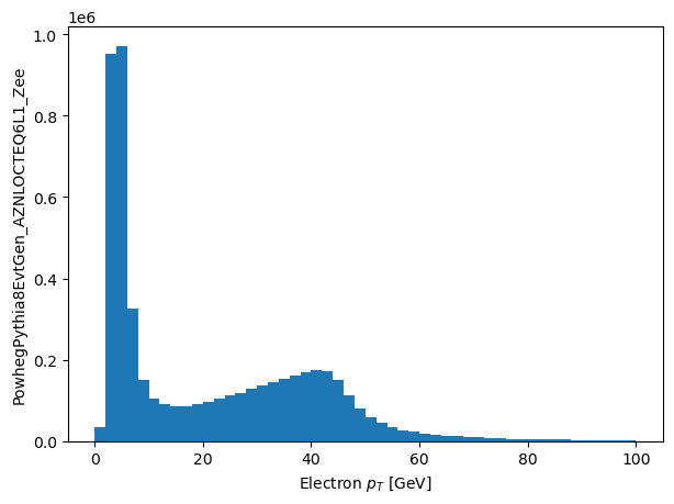
%%time
pts = df.Electrons("Electrons").pt/1000.0
This was instantanious because have built the DAG for extracting the electron $p_T$. If we want to plot it, we have to materalize it and bring the data local. Then we can plot it:
%%time
np_pts = make_local(pts)
The above cell did the following things:
- Translated the DAQ into a data-query expression for
servicex - Sent the query to
servicex.servicexran on 17 files that are in the $Z\rightarrow ee$ dataset, and collected their results. The package then downloaded the results locally. - Wrapped up the results as an in-memory JaggedArray.
plt.hist(np_pts.flatten(), range=(0, 100), bins=50)
plt.xlabel('Electron $p_T$ [GeV]')
_ = plt.ylabel('PowhegPythia8EvtGen_AZNLOCTEQ6L1_Zee')
The data that comes back is a very simple JaggedArray - this is from the awkward array package. So you can manipulate it as you normally would. Since we only pulled back the data we wanted, it is nice and small and easy to
print (type(np_pts))
print (np_pts.shape)
import awkward
awkward.topandas(np_pts, flatten=True)
Filtering Single Objects
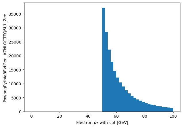
What if we only want to look at the electrons with a $p_T$ above 50 GeV? Then we use the slice operations that numpy and pandas have gotten us used to. To avoid repeating ourselves and typing long lines, it is convienient to define a few variables as short-cuts. We also want a list of good electrons, so lets define that.
%%time
eles = df.Electrons("Electrons")
good_eles = eles[(eles.pt > 50000.0) & (abs(eles.eta) < 1.5)]

np_pts_good_short = make_local(good_eles.pt/1000.0)
plt.hist(np_pts_good_short.flatten(), range=(0, 100), bins=50)
plt.xlabel('Electron $p_T$ with cut [GeV]')
_ = plt.ylabel('PowhegPythia8EvtGen_AZNLOCTEQ6L1_Zee')
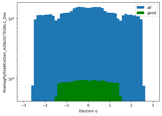
So now we can look at the $\eta$ distributions before and after that cut if we like. Note we move the lists right inside the make_local call as we aren't going to really need those definitions elsewhere.
%%time
np_eta_all = make_local(eles.eta)
np_eta_good = make_local(good_eles.eta)
plt.hist(np_eta_all.flatten(), label='all', bins=50, range=(-3.0,3.0))
plt.hist(np_eta_good.flatten(), label='good', bins=50, range=(-3.0,3.0), color='g')
plt.yscale('log')
plt.ylabel('PowhegPythia8EvtGen_AZNLOCTEQ6L1_Zee')
plt.xlabel('Electron $\eta$')
plt.legend();
Filter Functions
Sometimes filters can get a bit complex or you'd like to re-use them, or define them in one file and use them in another. Filter functions are a way to do that. The function is just inserted into the filter, and will, effectively, be called as if it has a single electron as an argument:
def central_good_ele(e):
    return (e.pt/1000.0 > 40) & (abs(e.eta) < 1.5)

central_good_eles = eles[central_good_ele]
%%time
np_eta_central_good = make_local(central_good_eles.eta)
plt.hist(np_eta_all.flatten(), label='all', bins=50, range=(-3.0,3.0))
plt.hist(np_eta_central_good.flatten(), label='central good', bins=50, range=(-3.0,3.0), color='y')
plt.hist(np_eta_good.flatten(), label='good', bins=50, range=(-3.0,3.0), color='g')
plt.yscale('log')
plt.ylabel('PowhegPythia8EvtGen_AZNLOCTEQ6L1_Zee')
plt.xlabel('Electron $\eta$')
plt.legend();
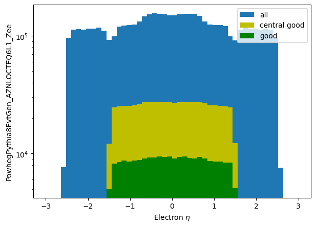
There isn't anything very magical occuring here: the function is called with an argument of whatever preceeds the filtering brackets. So eles[central_good_ele] is a short cut for eles[central_good_ele(eles)]. This is more about syntatic sugar.
Filtering on numbers of objects
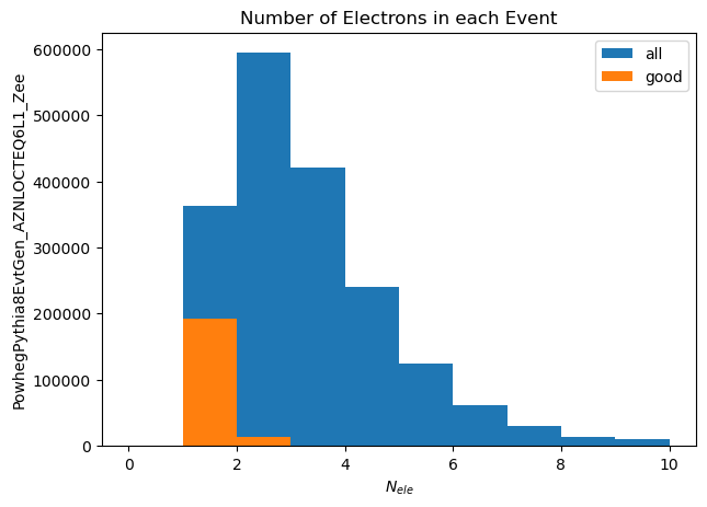
So far the selection and filtering has all been on a single object - like a single electron having $p_T > 50$ GeV. What if you want to require at least two electrons that satisfy that requirement? To count the number of objects that satisfy a requirement, after the cuts, add the Count() method. Count will always count the number of objects it is looking at. It can be used both to get back counts and also to filter:
%%time
electron_counts = make_local(eles.Count())
good_electron_counts = make_local(good_eles.Count())
plt.hist(electron_counts[electron_counts>0], label='all', range=(0,10))
plt.hist(good_electron_counts[good_electron_counts>0], label='good', range=(0,10))
plt.xlabel('$N_{ele}$')
plt.ylabel('PowhegPythia8EvtGen_AZNLOCTEQ6L1_Zee')
plt.title('Number of Electrons in each Event')
_ = plt.legend()
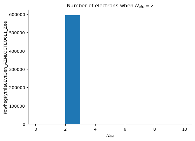
And we can also filter on number of electrons, creating a collection of events that have only two electrons:
%%time
good_events = df[eles.Count() == 2]
ele_per_event_count = make_local(good_events.Electrons("Electrons").Count())
plt.hist(ele_per_event_count, range=(0,10))
plt.title ('Number of electrons when $N_{ele} = 2$')
plt.xlabel('$N_{ele}$')
_ = plt.ylabel('PowhegPythia8EvtGen_AZNLOCTEQ6L1_Zee')