
This section takes you through some of the support in the current hep_tables package for calling functions:
- Math functions implemented by python (e.g.
abs) - Using
numpyfunctions on arrays, and usingnumpy.histogramon the backend. - The special
mapfunction, to apply a function to a sequence of values - Defining and calling arbitrary functions that are availible in the backend.
import sys
sys.path = ['..'] + sys.path
from hep_tables import xaod_table, make_local
from func_adl import EventDataset
import matplotlib.pyplot as plt

import numpy as np

plt.rcParams.update({'figure.figsize':(7,5), 'figure.dpi':100})
dataset = EventDataset('localds://mc15_13TeV:mc15_13TeV.361106.PowhegPythia8EvtGen_AZNLOCTEQ6L1_Zee.merge.DAOD_STDM3.e3601_s2576_s2132_r6630_r6264_p2363_tid05630052_00')
df = xaod_table(dataset)
Generic Math Functions
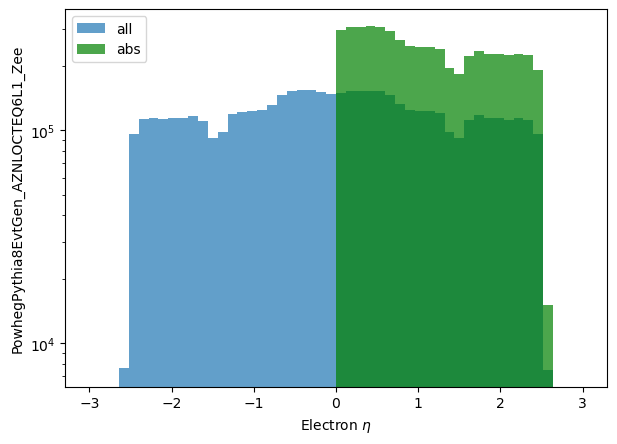
Python comes with a few math functions built in - that is, objects can directly support abs and the like. While only abs is implemented currently, you can see others that are possible in the python documentation. The abs function already appeared in the previous page looking at filtering for the electron's eta. Here it is again, in a simpler example:
%%time
eles = df.Electrons("Electrons")
np_eta_all = make_local(eles.eta)
np_eta_abs = make_local(abs(eles.eta))
plt.hist(np_eta_all.flatten(), label='all', bins=50, range=(-3.0,3.0), alpha=0.7)
plt.hist(np_eta_abs.flatten(), label='abs', bins=50, range=(-3.0,3.0), color='g', alpha=0.7)
plt.yscale('log')
plt.xlabel('Electron $\eta$')
plt.ylabel('PowhegPythia8EvtGen_AZNLOCTEQ6L1_Zee')
plt.legend();
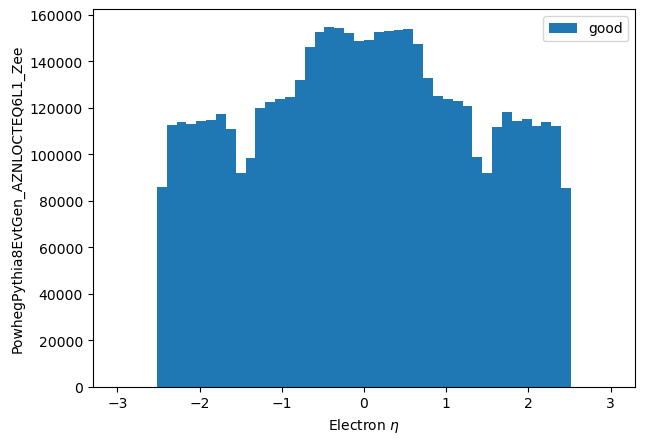
%%time
eles = df.Electrons("Electrons")
good_eles = eles[np.abs(eles.eta) < 2.5]
np_pts_good_short = make_local(good_eles.eta)
plt.hist(np_pts_good_short.flatten(), label='good', bins=50, range=(-3.0,3.0))
plt.xlabel("Electron $\eta$")
plt.ylabel('PowhegPythia8EvtGen_AZNLOCTEQ6L1_Zee')
plt.legend();
Histograms
When it comes down to it, in Run 4+, it is not likely we can run this locally on our home computer or laptop - we'll need to run it remotely. Unfortunately, numpy doesn't use the above extension mechanism for numpy.histogram. Here I've created a small histogram implementation that could run remotly. This was done by creating a simple histogram function and having it call numpy.histogram. As an example:
from hep_tables import histogram
good_eles = eles[np.abs(eles.eta) < 2.5]
good_ele_hist = make_local(histogram(good_eles.eta, bins=50, range=(-3.0,3.0)))
good_ele_hist
plt.plot(good_ele_hist[1][:-1], good_ele_hist[0], marker='o')
plt.ylabel('PowhegPythia8EvtGen_AZNLOCTEQ6L1_Zee')
plt.xlabel('Electron $\eta$')
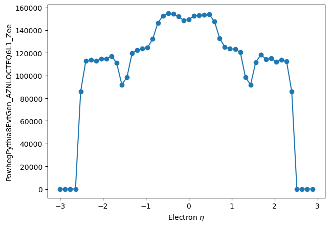
The servicex transformer we are talking to can't actually fill a histogram. So the following steps occured:
- We built a computational graph that included a call to the function
histogram. This was then handed to thehep_tablesbackend for processing. make_localpicked off the data that needed to be histogramed, and shipped it off toservicexas normal- It then uses the real
np.histogramto fill a histogram, and packaged up the results - And then shipped those back to the user.
- I demonstrated how badly I know
matplotlibwith that aweful looking histogram rather than understanding how to usematplotlibs'shistwith pre-binned data.
Other than the plotting, these instructions are in the computational graph before make_local is called - so could easily be shipped to a remote analysis facility. And one would imagine the histogram data being shipped in a more transportable format, like aghast.
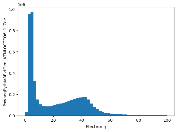
The map function
The map function is a common function that takes a sequence of values, like $seq = (x_0, x_1, x_2, x_3,...)$ and a single argument function like f(x), and applies them such that $map(f, seq) = (f(x_0), f(x_1), f(x_2), f(x_3), ...)$. In many places this map function has been effectively used already. For example, ele_pt = df.eles.pt could be written as:
df.eles.map(lambda e: e.pt)The map function is explicitly implemented in this prototype, and lends itself to a number of situations, as will be seen in a later section.
mapped_eles = eles.map(lambda e: e.pt/1000.0)
%%time
mapped_eles_pt = make_local(mapped_eles)
plt.hist(mapped_eles_pt.flatten(), bins=50, range=(0, 100.0))
plt.ylabel('PowhegPythia8EvtGen_AZNLOCTEQ6L1_Zee')
_ = plt.xlabel('Electron $\eta$')
Now that the concept is down, much more complex things are possible inside that lambda. And there is no need for it to be a lambda - it can be a normal function as long as it returns a calculated expressions (so no if statements on data, etc.). The real power of this will be seen when we look at multiple objects in one expression later on.
Backend Functions (leaky abstractions)
There are times one wants to use a stand-alone function that is availible at the backend. This is one example of a leaky abstraction. hep_tables uses a fairly simple syntax to declare a function like this. For example, in the current ATLAS xAOD servicex transformer the DeltaR function is declared, which is a lazy way of calculating $\Delta R$ between two objects.
The first step is to declare the function to the hep_tables backend using a decorator. That way when it is encountered, hep_tables will know to pass it through untouched to the servicex backend.
from dataframe_expressions import user_func

@user_func
def DeltaR(p1_eta: float, p1_phi: float, p2_eta: float, p2_phi: float) -> float:
    '''
    Calculate the DeltaR between two particles given their `eta` and `phi` locations.
    Implemented on the back end.
    '''
    assert False, 'This should never be called'
The type hints are used to make sure a mistake hasn't occured: I'm trying to be better. The decorator user_func declares it to the system as a function that should be called on the back end. We can now use it - although in a rather boring example:
mapped_eles = eles.map(lambda e: DeltaR(e.eta, e.phi, e.eta, e.phi))
%%time
delta_r_zero = make_local(mapped_eles)
delta_r_zero